Use of these data is subject to the WDC Kyoto data usage rules — see also Rules of the road for how to credit the data. Please cite the indices by their DOIs:
| Dst | doi:10.17593/14515-74000 |
|---|---|
| AE | doi:10.17593/15031-54800 |
| ASY/SYM | doi:10.14989/267216 |
| Kp / ap / Ap | doi:10.5880/Kp.0001 — GFZ Potsdam |
This server of the World Data Center for Geomagnetism, Kyoto supports the HAPI 3.3.1 API specification for delivery of time series data. It serves geomagnetic indices (Dst, AE, ASY/SYM, Kp/ap) and geomagnetic field observatory data (hourly, 1-minute, 7.5-second and 1-second values). The server responds to GET requests to the following HAPI endpoints:
capabilities— list the API version and the supported output formatsabout— list the server ID, title and contact informationcatalog— list every dataset this server servesinfo— describe the parameters, time range and metadata of one datasetdata— stream the time series data for a dataset and time range
One further endpoint is a non-standard extension, outside the HAPI specification, added for the Data Explorer and free to use:
availability— list the time intervals for which source files exist, for every dataset (or for one, with?dataset=<id>).infoadvertises only the first and last timestamp, so a dataset with a break in the middle looks continuous there; this endpoint shows the break. A covered interval means the source files are present, not that every timestamp in it has a value.
Open the Geomagnetic Data Explorer — plot & download in your browser →
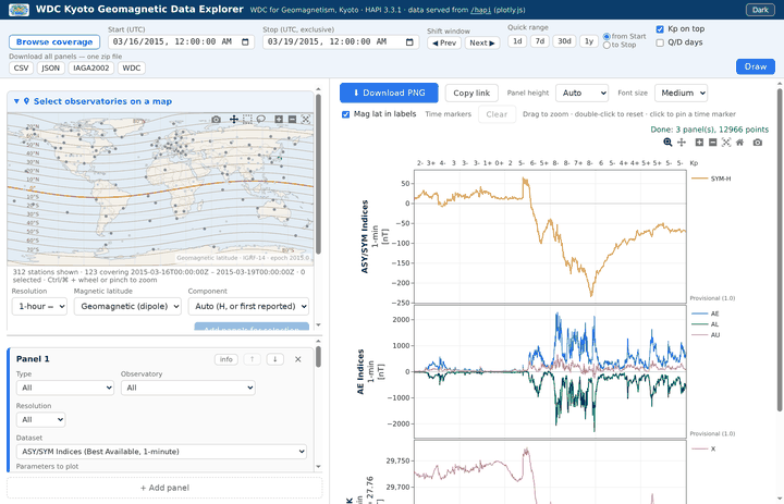 Example: SYM-H, AE and Kakioka X for the storm of
17 March 2015 — click to open it.
Example: SYM-H, AE and Kakioka X for the storm of
17 March 2015 — click to open it.
No code required: pick datasets and a time range, view them as stacked panels, and download the result as CSV, JSON, IAGA-2002 or WDC (format descriptions). Observatories can also be picked on a world map or by a latitude/longitude box, which adds one panel per station in a single step. Prefer Python? See Reading the data from Python.
Available datasets
These are the Best Available datasets — the IDs without a version
suffix. Each one always serves the highest processing level that exists for a
given time, and the versionCode parameter records which level every
record came from. These are the datasets to use.
Which levels exist depends on the dataset. The Dst and AE indices run
Real-time (0) → Provisional (1) → Final (2); the Kp-derived indices
(hour3h_kp, day_ap, month_qddays)
currently have a single definitive version. Observatory datasets follow the
IAGA2002 Data Type levels — Variation (0) → Provisional (1) →
Quasi-definitive (2) → Definitive (3); hourly, 1-minute and 1-second values are
served as Definitive, the 7.5-second values as Quasi-definitive, and the
sec_kyo_* monitor stations as Real-time (0).
Each dataset’s info response documents the codes that apply
to it, in the description of its versionCode parameter.
The list below is a summary; catalog is
authoritative.
| Group | Dataset ID | Title |
|---|---|---|
| Indices | hour_dst | Dst Index (Best Available, 1-hour) |
hour_ae | AE Indices (Best Available, 1-hour) | |
min_ae | AE Indices (Best Available, 1-minute) | |
min2p5_ae | AE Indices (Best Available, 2.5-minute) | |
min_asysym | ASY/SYM Indices (Best Available, 1-minute) | |
hour3h_kp | Kp and ap Indices (Best Available, 3-hour) | |
day_ap | Ap Index (Best Available, daily) | |
month_qddays | International Quiet and Disturbed Days (Best Available, monthly) | |
| Observatories | min_<obs> (e.g. min_kak) | <obs> Observatory (Best Available, 1-minute) |
min_<obs>_definitive | <obs> Observatory (Definitive, 1-minute) | |
hour_<obs> (e.g. hour_kak) | <obs> Observatory (Best Available, 1-hour) | |
hour_<obs>_definitive | <obs> Observatory (Definitive, 1-hour) | |
sec7p5_<obs> (e.g. sec7p5_kak) | <obs> Observatory (Best Available, 7.5-second) — KAK, KNY and MMB only (1956–1984) | |
sec7p5_<obs>_quasidefinitive | <obs> Observatory (Quasi-definitive, 7.5-second) | |
sec_<obs> (e.g. sec_kak) | <obs> Observatory (Best Available, 1-second) — 13 observatories (1978–2026) | |
sec_<obs>_definitive | <obs> Observatory (Definitive, 1-second) | |
| WDC Kyoto monitor stations |
sec_kyo_<stn> (e.g. sec_kyo_mya) | <stn> Station (Real-time, 1-second) — agw, mya, nks, onn, phi, sga (2009–2023). See the caution below |
sec_kyo_<stn>_press (e.g. sec_kyo_mya_press) | <stn> Station atmospheric pressure (Real-time, 1-second) — see the caution below |
Observatories — hour_<obs>,
min_<obs>, sec7p5_<obs>,
sec_<obs>
<obs> is the lower-case IAGA code of an observatory
(kak, abg, ngk, …); in the titles
above it stands for that observatory’s name, so min_kak is
titled Kakioka Observatory (Best Available, 1-minute). Hourly values are
served for 313 observatories covering 1844–2026, 1-minute values for
182 observatories, 7.5-second values for kak,
kny and mmb only (1956–1984, digitised from
magnetograms), and 1-second values for 13 observatories (1978–2026).
All observatory datasets carry the same seven columns
(D, H, X, Y, Z, F, I) and report the components exactly as the source
did — no coordinate conversion — so components not reported in a given
period are filled. See catalog for the
authoritative list.
WDC Kyoto monitor stations
— sec_kyo_<stn> and
sec_kyo_<stn>_press only
1-second variation data from 6 real-time monitor stations
operated by WDC for Geomagnetism, Kyoto are served as
sec_kyo_<stn> (Agawa agw, Mineyama
mya, Nakanoshima nks, Onna onn, Phimai
phi, Shigaraki sga; 2009–2023). These differ in
nature from the observatory datasets above and carry their own four columns
(H, E, Z, F, where E is the magnetic eastward variation
in nT). All currently served data are Real-time (versionCode 00).
Caution (monitor stations) — read before use.
H, E and Z are variation
components: the baseline is not accurate and is not controlled over time, so
they are not absolute field measurements. At some stations no baseline is
added at all — H is then only of the order of tens to hundreds
of nT — while at others only an approximate value has been added. The
source’s approximate baseline for each station is reproduced in the comment
block of the format=iaga2002 output, together with this caution. Use
these data for variations, not for absolute levels, and do not compare levels
between stations or across time without establishing your own baseline.
(F, where served, is an independent scalar measurement and is
absolute.)
The source supplies an approximate baseline per station
(Approx. D / Approx. H, reproduced in the comment block
of the format=iaga2002 output) for transforming the reported
elements: D is needed to transform the HEZ variation data to the
widely used XYZ orientation, and H to convert
E-variations in nT to variations in minutes of arc.
The data were collected for real-time monitoring and are served as recorded
— no noise removal, spike rejection or baseline control has been applied
— and timestamps may be inaccurate during periods when GPS timing or
the network connection was unavailable and the recording PC’s clock was
used instead.
The same stations also record atmospheric pressure alongside the field,
served separately as sec_kyo_<stn>_press (1-second, hPa). It is
kept out of the field datasets because it is a different physical quantity: mixing
hPa into a nT time series would break the axes of any plot and the meaning of a
bulk download, and the four-column IAGA2002 frame has no room for it. In
format=iaga2002 these datasets declare themselves
IAGA-2002-like (atmospheric pressure) with a single
P column, since a pressure column is outside the format.
Caution (monitor-station pressure). This is the pressure measured at the station’s own altitude and is not reduced to sea level, so the level reflects the station’s elevation and must not be compared between stations. The absolute accuracy of the barometer is not guaranteed and is not controlled over time, so the data must not be used to derive long-term trends; periods where the reading is stuck at a nearly constant value do occur, and at some stations the barometer failed for months at a time. As with the field, the data are served as recorded with no spike rejection or quality control, and the same timestamp caution applies. What they are good for is pressure variations at 1-second sampling — atmospheric gravity waves, Lamb waves and microbarometric oscillations — a cadence that routine meteorological observations do not provide.
Request limits — all datasets
A single data request is limited to 3 days for 1-second values,
31 days for 7.5-second values, 366 days for 1-minute values and 50 years for
observatory hourly values; the index datasets have no limit. Each
dataset’s info gives its own limit as
maxRequestDuration, and longer ranges return status
1408.
Version-pinned datasets — all groups above
Version-pinned datasets also exist, named after the level they serve
(hour_dst_final, hour_dst_provisional,
hour_dst_realtime and the equivalents for the other datasets); see
catalog for the full list. Each serves a
single processing level, so for any period where a higher level has since been
derived, they return the superseded values rather than the current ones. The
lower levels in particular — real-time and provisional — are
preliminary and are revised later.
Pinned versions are for traceability — reproducing exactly what a given version contained at a given time, for example to check a figure in an older paper. They are not the right choice for new scientific analysis: use the Best Available datasets above instead, which give the same values wherever no better version exists. If your use case really does call for a pinned version, and in particular before publishing results based on one, please contact us first.
Example queries
The links below are full URLs you can open directly in a browser. Data examples
use format=json so the response is shown as text in the browser;
append &format=csv instead to get CSV (which browsers usually
download as a file).
Metadata
Data
Reading the data from Python
hapiclient
is the reference HAPI client for Python. It handles paging, parsing and time
conversion, so a dataset is one call away:
pip install hapiclientfrom hapiclient import hapi
SERVER = 'https://wdc.kugi.kyoto-u.ac.jp/hapi'
# Dst index during the March 2015 (St. Patrick's Day) storm
data, meta = hapi(SERVER, 'hour_dst', 'dstValue',
'2015-03-16T00:00:00Z', '2015-03-19T00:00:00Z')
print(data[:3])
# [(b'2015-03-16T00:29:30Z', 4) (b'2015-03-16T01:29:30Z', 10)
# (b'2015-03-16T02:29:30Z', 15)]
data is a NumPy structured array and meta is the
info response. To get a pandas DataFrame with the fill
values (99999) turned into NaN:
import numpy as np, pandas as pd

fills = {p['name']: p.get('fill') for p in meta['parameters']}
df = pd.DataFrame(data)
df['Time'] = pd.to_datetime(df['Time'].str.decode('utf-8'), format='ISO8601')
df = df.set_index('Time')
for name, fill in fills.items():
    if name in df.columns and fill is not None:
        df[name] = df[name].astype('float64').replace(float(fill), np.nan)

df['dstValue'].plot()
Calling hapi(SERVER) returns the catalog and
hapi(SERVER, 'hour_dst') the metadata alone. The native
iaga2002 / wdc formats are not handled by
hapiclient; request those directly with
requests.get(SERVER + '/data', params={...}).
Runnable notebook — catalog browsing, Dst / AE / Kp plots,
fill-value handling, versionCode and native formats:
 or download it directly:
examples.ipynb
(for local Jupyter, or Colab’s File → Upload notebook).
or download it directly:
examples.ipynb
(for local Jupyter, or Colab’s File → Upload notebook).
SPEDAS and PySPEDAS
These datasets are also reachable from SPEDAS and PySPEDAS through the IUGONET plugins, which load them straight into tplot variables, so WDC Kyoto data sit alongside satellite and other ground-based data in the same analysis session. Both plugins are at github.com/iugonet — UDAS for SPEDAS (IDL) and pyudas for PySPEDAS — and take the same keywords on both sides:
; SPEDAS (IDL). Put the UDAS repository's iugonet/ directory on !path, ahead
; of the older copy that came with SPEDAS.
timespan, '2015-03-16', 3, /days
iug_load_gmag_wdc, site = ['dst', 'kak'], resolution = 'hour'
# PySPEDAS. pip install "git+https://github.com/iugonet/pyudas.git"
import iugonet
from pyspedas import tplot
iugonet.gmag_wdc(trange=['2015-03-16', '2015-03-19'],
site=['dst', 'kak'], resolution='hour')
tplot(['wdc_mag_dst', 'wdc_mag_kak_1hr'])Both plugins keep what they download as files on your own machine and reuse them on the next run, fetching a chunk again only when the server reports it has changed.
Notes
- Output formats:
csv(default) andjson. The geomagnetic index time series (Dst, AE, ASY/SYM) and the observatory data are also served in their nativeiaga2002andwdcformats (7.5-second and 1-second values have no WDC layout, so they supportiaga2002but notwdc); the Kp-derived indices (hour3h_kp,day_ap,month_qddays) supportcsv/jsononly. The layout of each format is described on the Output formats page. - Restrict the returned columns with
¶meters=, e.g.¶meters=alValue,auValue. - Time stamps mark the center of each averaging interval
(
timeStampLocation=center): hourly Dst values are stampedHH:29:30, 1-minute values are centered on the UT minute, 3-hourly Kp/ap at01:30, 04:30, … 22:30, and daily Ap at12:00. The monthlymonth_qddaysinstead marks the start of the month (YYYY-MM-01T00:00:00Z,timeStampLocation=begin). - Kp is given as a decimal where the plus/minus thirds map to fractional parts
.3and.7(e.g. 3−=2.7, 3o=3.0, 3+=3.3). - Both HAPI 3 (
dataset/start/stop) and HAPI 2 (id/time.min/time.max) request parameter names are accepted.
Magnetograms
 A magnetogram in COMPASS — click to open the
portal.
A magnetogram in COMPASS — click to open the
portal.
This server delivers digital time series only. The magnetogram images — the analog records the early observatory data were read from — are served by a companion WDC Kyoto service, COMPASS (Comprehensive Magnetogram Portal and Archive Service System). COMPASS is to the images what this server is to the data: about 1.4 million digitised magnetograms and tellurigrams from observatories around the world, published through the IIIF image API, so a sheet can be browsed at high resolution in the viewer, downloaded at original quality, or pulled into any IIIF client.